「修炼开始」一文带你入门深度学习

一、前言

承诺的图解 AI 算法系列教程，今天它来了！

最近，写了很多 AI 趣味性算法教程，目前写了 14 篇，其中反响不错的教程有：

• 你的红色高跟鞋，AI 换脸技术初体验
• 让图片动起来，特朗普和蒙娜丽莎深情合唱《Unravel》
• 为艺术而生的惊艳算法
• 百年老照片修复算法，那些高颜值的父母！
• 「完美复刻」的人物肖像画生成算法 U^2-Net

读者们玩得很开心，对 AI 算法、深度学习也来了兴趣。

但仅限于开心地跑包，这最多只能算是「调包侠」。

既然来了兴致，何不趁热打铁，多学些基础知识，争取早日迈入「调参侠」的行列。

大家一起炼丹，一起修炼。

图解 AI 算法系列教程，不仅仅是涉及深度学习基础知识，还会有强化学习、迁移学习等，再往小了讲就比如拆解目标检测算法，对抗神经网络（GAN）等等。

难度会逐渐增加，今天咱先热热身，来点轻松的，当作这个系列的开篇。

二、深度学习

想学深度学习，要掌握哪些基础知识？直接上图：

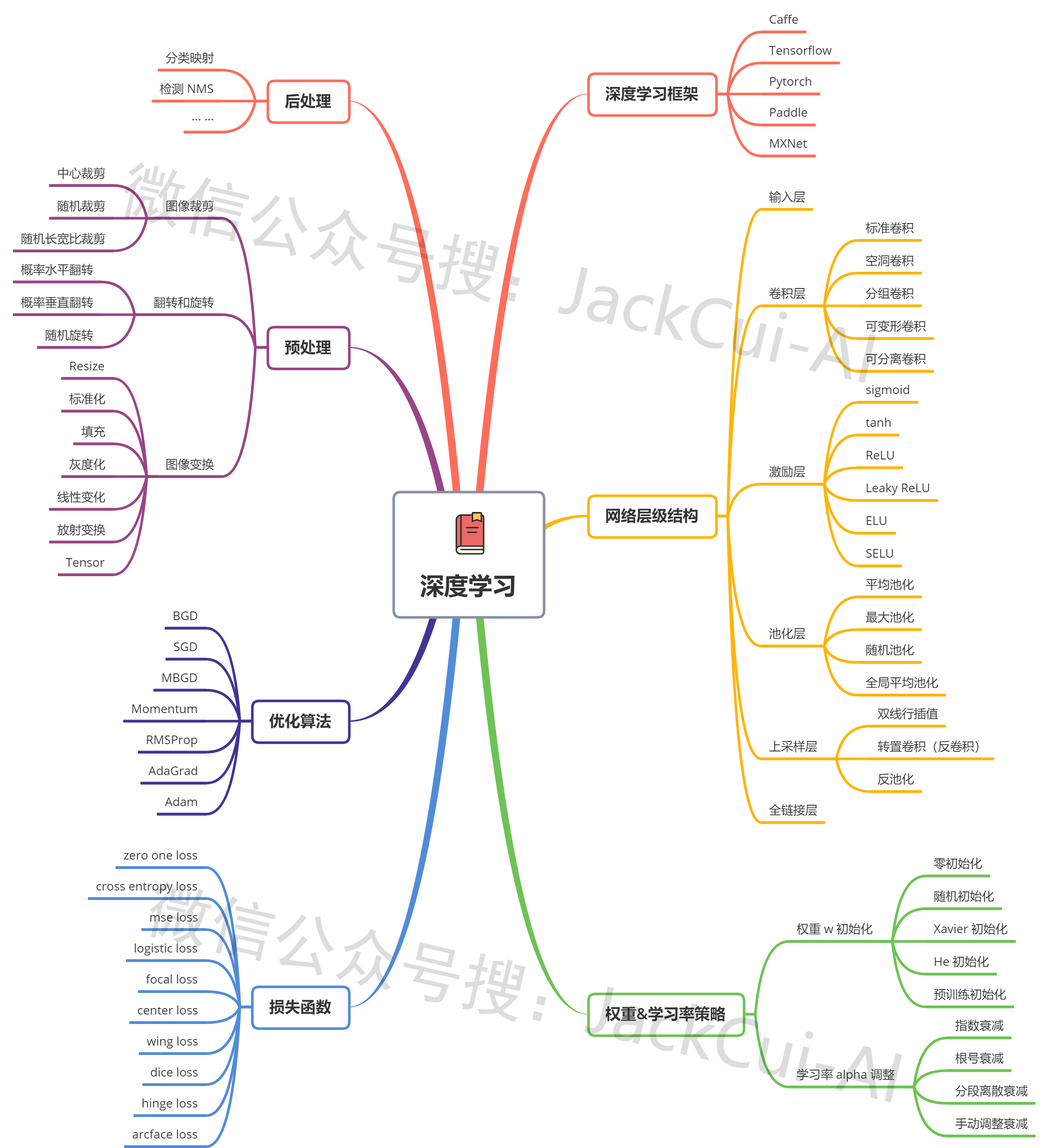
整理了小半天的思维导图，建议收藏！

深度学习主要由上图所示的几个部分组成，想学一个深度学习算法的原理，就看它是什么样的网络结构，Loss 是怎么计算的，预处理和后处理都是怎么做的。

权重初始化和学习率调整策略、优化算法、深度学习框架就那么多，并且也不是所有都要掌握，比如深度学习框架，Pytorch 玩的溜，就能应付大多数场景。

先有个整体的认知，然后再按照这个思维导图，逐个知识点学习，最后整合到一起，你会发现，你也可以自己实现各种功能的算法了。

深度学习的主要目的是从数据中自动学习到有效的特征表示，它是怎么工作的？那得从神经元说起。

随着神经科学、认知科学的发展，我们逐渐知道人类的智能行为都和大脑活动有关。

人脑神经系统^[1]是一个非常复杂的组织，包含近 860 亿个神经元，这 860 亿的神经元构成了超级庞大的神经网络。

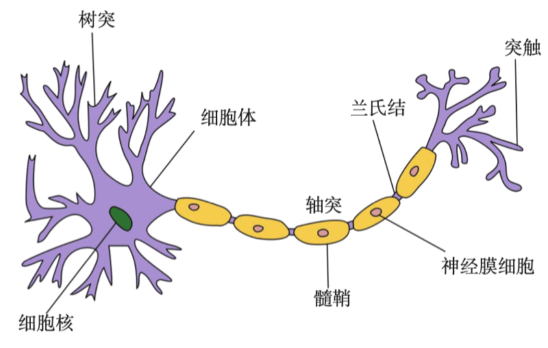
我们知道，一个人的智力不完全由遗传决定，大部分来自于生活经验。也就是说人脑神经网络是一个具有学习能力的系统。

不同神经元之间的突触有强有弱，其强度是可以通过学习（训练）来不断改变的，具有一定的可塑性，不同的连接又形成了不同的记忆印痕。

而深度学习的神经网络，就是受人脑神经网络启发，设计的一种计算模型，它从结构、实现机理和功能上模拟人脑神经网络。

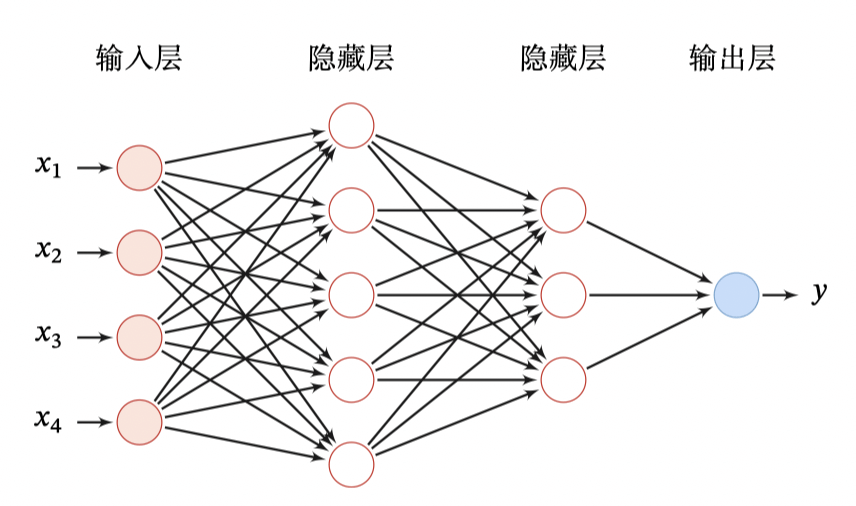
比如下图就是一个最简单的前馈神经网络，第 0 层称为输入层，最后一层称为输出层，其他中间层称为隐藏层。

那神经网络如何工作的？网络层次结构、损失函数、优化算法、权重初始化、学习率调整都是如何运作的？

反向传播给你答案。前方，高能预警！

三、反向传播

要想弄懂深度学习原理，必须搞定反向传播^[2]和链式求导法则。

先说思维导图里的网络层级结构，一个神经网络，可复杂可简单，为了方便推导，假设，你有这样一个网络层：

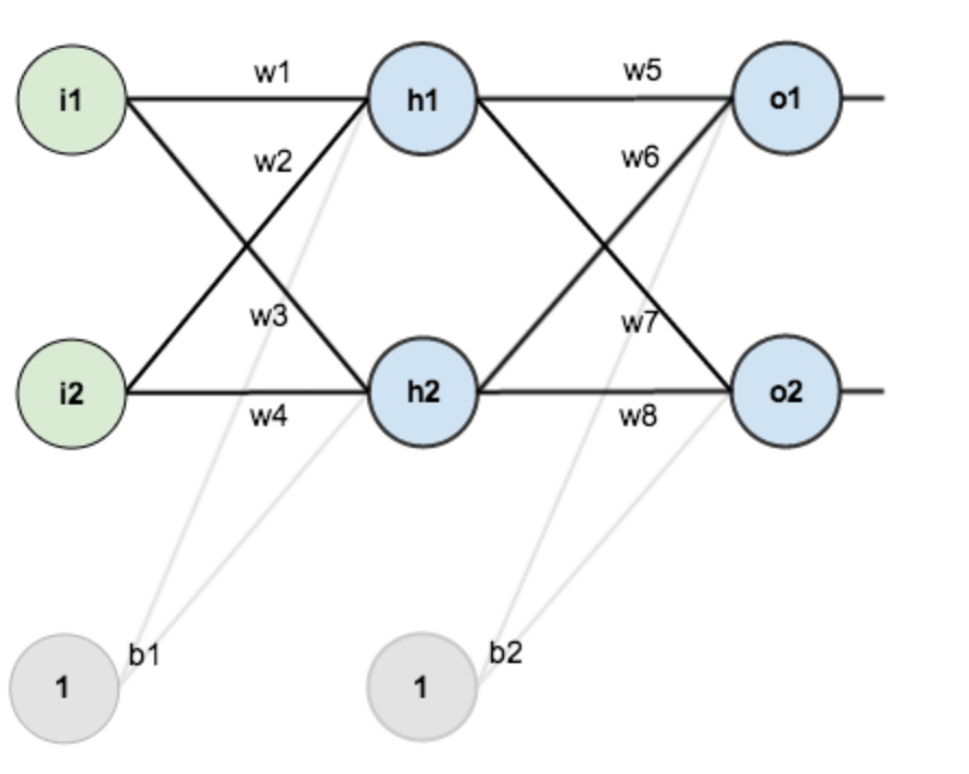
第一层是输入层，包含两个神经元 i1, i2 和截距项 b1（偏置）；

第二层是隐含层，包含两个神经元 h1, h2 和截距项 b2 ；

第三层是输出层 o1 和 o2 ，每条线上标的 wi 是层与层之间连接的权重，激活函数我们默认为 sigmoid 函数。

在训练这个网络之前，需要初始化这些 wi 权重，这就是权重初始化，这里就有不少的初始化方法，我们选择最简单的，随机初始化。

随机初始化的结果，如下图所示：

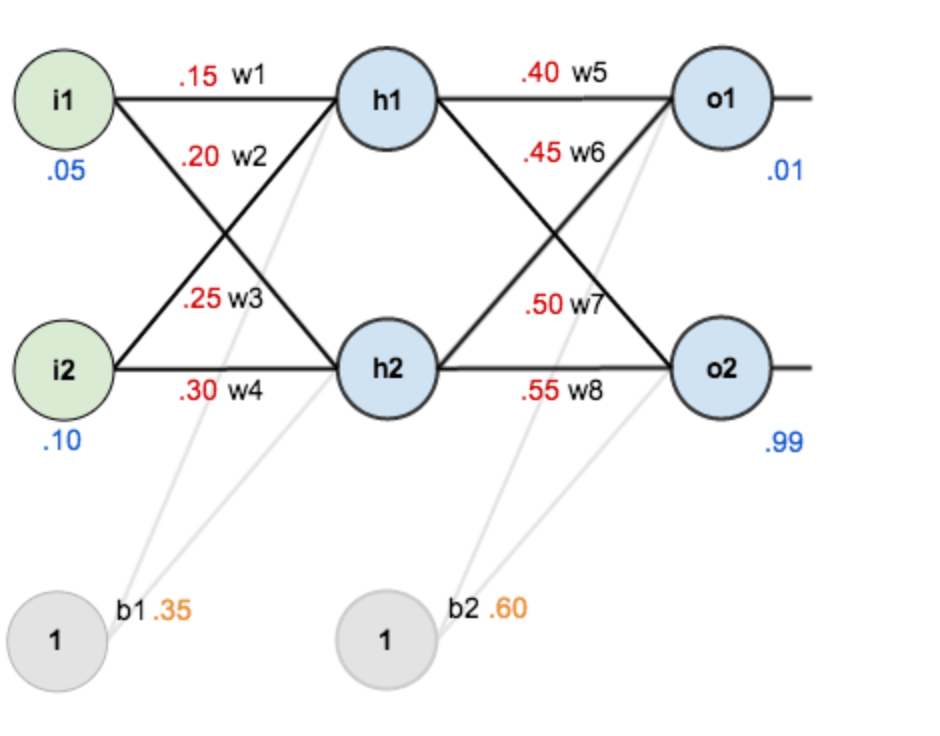
其中，输入数据: i1=0.05, i2=0.10;

输出数据（期望的输出） : o1=0.01, o2=0.99;

初始权重: w1=0.15, w2=0.20, w3=0.25, w4=0.30, w5=0.40, w6=0.45, w7=0.50, w8=0.55。

目标：给出输入数据 i1, i2(0.05 和 0.10)，使输出尽可能与原始输出o1, o2(0.01 和 0.99)接近。

神经网络的工作流程分为两步：前向传播和反向传播。

1、前向传播

前向传播是将输入数据根据权重，计算到输出层。

1）输入层->隐藏层

计算神经元 h1 的输入加权和：

$$
\begin{array}{l}
\text { net }_{h 1}=w_{1} * i_{1}+w_{2} * i_{2}+b_{1} * 1 \\
\text { net }_{h 1}=0.15 * 0.05+0.2 * 0.1+0.35 * 1=0.3775
\end{array}
$$

神经元后面，要跟个激活层，从而引入非线性因素，这就像人的神经元一样，让细胞处于兴奋或抑制的状态。

数学模拟的形式就是通过激活函数，大于阈值就激活，反之抑制。

常用的激活函如思维导图所示，这里以非常简单的 sigmoid 激活函数为例，它的函数形式如下：

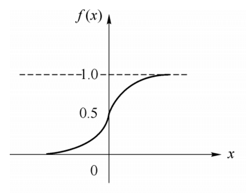
数学公式：

$$
f(x) = \frac{1}{1+e^{-x}}
$$

使用 sigmoid 激活函数，继续计算，神经元 h1 的输出 o_h1：

$$
\text { out }_{h 1}=\frac{1}{1+e^{-n e t_{h 1}}}=\frac{1}{1+e^{-0.3775}}=0.593269992
$$

同理，可计算出神经元 h2 的输出 o_h2：

$$
\text { out }_{h 2}=0.596884378
$$

2）隐藏层->输出层

计算输出层神经元 o1 和 o2 的值：

$$
\begin{array}{l}
\text { net }_{o 1}=w_{5} * \text { out }_{h 1}+w_{6} * \text { out }_{h 2}+b_{2} * 1 \\
\text { net }_{o 1}=0.4 * 0.593269992+0.45 * 0.596884378+0.6 * 1=1.105905967 \\
\text { out }_{o 1}=\frac{1}{1+e^{-n e t_{o 1}}}=\frac{1}{1+e^{-1.105905967}}=0.75136507
\end{array}
$$

这样前向传播的过程就结束了，根据输入值和权重，我们得到输出值为[0.75136079, 0.772928465]，与实际值（目标）[0.01, 0.99]相差还很远，现在我们对误差进行反向传播，更新权值，重新计算输出。

2、反向传播

前向传播之后，发现输出结果与期望相差甚远，这时候就要更新权重了。

所谓深度学习的训练（炼丹），学的就是这些权重，我们期望的是调整这些权重，让输出结果符合我们的期望。

而更新权重的方式，依靠的就是反向传播。

1）计算总误差

一次前向传播过后，输出值（预测值）与目标值（标签值）有差距，那得衡量一下有多大差距。

衡量的方法，就是用思维导图中的损失函数。

损失函数也有很多，咱们还是选择一个最简单的，均方误差（MSE loss）。

均方误差的函数公式：

$$
M S E=\frac{1}{n} \sum_{i=1}^{n}\left(\hat{y}_{i}-y_{i}\right)^{2}
$$

根据公式，直接计算预测值与标签值的总误差：

$$
E_{\text {total}}=\sum \frac{1}{2}(\text {target}-\text {output})^{2}
$$

有两个输出，所以分别计算 o1 和 o2 的误差，总误差为两者之和：

$$
\begin{array}{l}
E_{o 1}=\frac{1}{2}\left(\text {target}_{o 1}-\text {out}_{o 1}\right)^{2}=\frac{1}{2}(0.01-0.75136507)^{2}=0.274811083 \\
E_{o 2}=0.023560026 \\
E_{\text {total}}=E_{o 1}+E_{o 2}=0.274811083+0.023560026=0.298371109
\end{array}
$$

2）隐含层->输出层的权值更新

以权重参数 w5 为例，如果我们想知道 w5 对整体误差产生了多少影响，可以用整体误差对 w5 求偏导求出。

这是链式法则，它是微积分中复合函数的求导法则，就是这个：

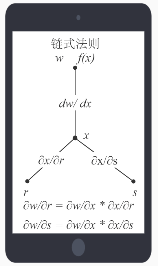
根据链式法则易得：

$$
\frac{\partial E_{\text {total}}}{\partial w_{5}}=\frac{\partial E_{\text {total}}}{\partial \text {out}_{o 1}} * \frac{\partial \text {out}_{o 1}}{\partial \text {net}_{o 1}} * \frac{\partial \text {net}_{o 1}}{\partial w_{5}}
$$

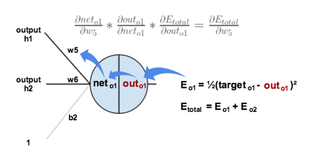
下面的图可以更直观的看清楚误差是怎样反向传播的：

现在我们来分别计算每个式子的值：

计算\(\frac{\partial E_{\text {total}}}{\partial \text {out}_{o 1}}\)：

$$
E_{\text {total}}=\frac{1}{2}\left(\text {target}_{o 1}-\text {out}_{o 1}\right)^{2}+\frac{1}{2}\left(\text {target}_{o 2}-\text {out}_{o 2}\right)^{2}
$$

$$
\frac{\partial E_{\text {tatal}}}{\partial o u t_{o 1}}=2 * \frac{1}{2}\left(\text {target}_{o 1}-\text {out}_{o 1}\right)^{2-1} *-1+0
$$

$$
\frac{\partial E_{\text {tatal }}}{\partial \text { out }_{\text {ol }}}=-\left(\text { target }_{\text {ol }}-\text { out }_{\text {ol }}\right)=-(0.01-0.75136507)=0.74136507
$$

计算\(\frac{\partial o u t_{o 1}}{\partial n e t_{o 1}}\):

$$
\begin{array}{l}
\text {out}_{o 1}=\frac{1}{1+e^{-n e t_{o 1}}} \\
\frac{\partial o u t_{o 1}}{\partial n e t_{o 1}}=o u t_{o 1}\left(1-o u t_{o 1}\right)=0.75136507(1-0.75136507)=0.186815602
\end{array}
$$

这一步实际上就是对sigmoid函数求导，比较简单，可以自己推导一下。

计算\(\frac{\partial n e t_{o 1}}{\partial w_{5}}\)：

$$
\begin{array}{l}
\text { net }_{o 1}=w_{5} * \text { out }_{h 1}+w_{6} * \text { out }_{h 2}+b_{2} * 1 \\
\frac{\partial n e t_{o 1}}{\partial w_{5}}=1 * \text { out }_{h 1} * w_{5}^{(1-1)}+0+0=\text { out }_{h 1}=0.593269992
\end{array}
$$

最后三者相乘：

$$
\frac{\partial E_{\text {total}}}{\partial w_{5}}=\frac{\partial E_{\text {total}}}{\partial o u t_{o 1}} * \frac{\partial \text {out}_{o 1}}{\partial n e t_{o 1}} * \frac{\partial n e t_{o 1}}{\partial w_{5}}
$$

$$
\frac{\partial E_{t t a l}}{\partial w_{5}}=0.74136507 * 0.186815602 * 0.593269992=0.082167041
$$

这样我们就计算出整体误差E(total)对 w5 的偏导值。

回过头来再看看上面的公式，我们发现：

$$
\frac{\partial E_{\text {tatal }}}{\partial u_{5}}=-\left(\text {target}_{o 1}-\text { out }_{\text {ol }}\right) * \text { out }_{\text {ol }}\left(1-\text { out }_{\text {ol }}\right) * \text { out }_{h 1}
$$

为了表达方便，用\(\delta_{o 1}\)来表示输出层的误差：

$$
\delta_{o 1}=\frac{\partial E_{\text {total }}}{\text { dout }_{\text {ol }}} * \frac{\text { dout }_{\text {ol }}}{\text { Onet }_{\text {ol }}}=\frac{\partial E_{\text {total }}}{\text { onet }_{\text {ol }}}
$$

$$
\delta_{o 1}=-\left(\text {target}_{o 1}-o u t_{o 1}\right) * \text { out }_{o 1}\left(1-\text { out }_{o 1}\right)
$$

因此，整体误差E(total)对w5的偏导公式可以写成：

$$
\frac{\partial E_{\text {total}}}{\partial w_{5}}=\delta_{o 1} \text { out }_{h 1}
$$

如果输出层误差计为负的话，也可以写成：

$$
\frac{\partial E_{t o t a l}}{\partial w_{5}}=-\delta_{o 1} \text { out }_{h 1}
$$

最后我们来更新 w5 的值：

$$
w_{5}^{+}=w_{5}-\eta * \frac{\partial E_{t o t a l}}{\partial w_{5}}=0.4-0.5 * 0.082167041=0.35891648
$$

这个更新权重的策略，就是思维导图中的优化算法，

η

 是学习率，我们这里取0.5。

如果学习率要根据迭代的次数调整，那就用到了思维导图中的学习率调整。

同理，可更新w6,w7,w8:

$$
\begin{array}{l}
w_{6}^{+}=0.408666186 \\
w_{7}^{+}=0.511301270 \\
w_{8}^{+}=0.561370121
\end{array}
$$

3）隐含层->隐含层的权值更新

方法其实与上面说的差不多，但是有个地方需要变一下，在上文计算总误差对 w5 的偏导时，是从out(o1)->net(o1)->w5，但是在隐含层之间的权值更新时，是out(h1)->net(h1)->w1,而 out(h1) 会接受 E(o1) 和 E(o2) 两个地方传来的误差，所以这个地方两个都要计算。

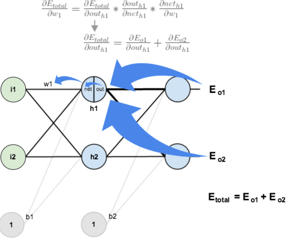
计算\(\frac{\partial E_{\text {total}}}{\partial \text {out}_{h 1}}\)：

$$
\frac{\partial E_{\text {total}}}{\partial o u t_{h 1}}=\frac{\partial E_{o 1}}{\partial o u t_{h 1}}+\frac{\partial E_{o 2}}{\partial o u t_{h 1}}
$$

先计算\(\frac{\partial E_{o 1}}{\partial o u t_{h 1}}\):

$$
\begin{array}{l}
\frac{\partial E_{o 1}}{\partial o u t_{h 1}}=\frac{\partial E_{o 1}}{\partial n e t_{o 1}} * \frac{\partial n e t_{o 1}}{\partial o u t_{h 1}} \\
\frac{\partial E_{o 1}}{\partial n e t_{o 1}}=\frac{\partial E_{o 1}}{\partial o u t_{o 1}} * \frac{\partial o u t_{o 1}}{\partial n e t_{o 1}}=0.74136507 * 0.186815602=0.138498562 \\
\text { net }_{o 1}=w_{5} * \text { out }_{h 1}+w_{6} * \text { out }_{h 2}+b_{2} * 1 \\
\frac{\partial n e t_{o 1}}{\partial o u t_{h 1}}=w_{5}=0.40 \\
\frac{\partial E_{o 1}}{\partial o u t_{h 1}}=\frac{\partial E_{o 1}}{\partial n e t_{o 1}} * \frac{\partial n e t_{o 1}}{\partial o u t_{h 1}}=0.138498562 * 0.40=0.055399425
\end{array}
$$

同理，计算出：

$$
\frac{\partial E_{o 2}}{\partial o u t_{h 1}}=-0.019049119
$$

两者相加得到总值：

$$
\frac{\partial E_{\text {total}}}{\partial o u t_{h 1}}=\frac{\partial E_{o 1}}{\partial o u t_{h 1}}+\frac{\partial E_{o 2}}{\partial o u t_{h 1}}=0.055399425+-0.019049119=0.036350306
$$

再计算\(\frac{\partial o u t_{h 1}}{\partial n e t_{h 1}}\):

$$
\begin{array}{l}
\text { out }_{h 1}=\frac{1}{1+e^{-n e t} t_{h 1}} \\
\frac{\text { out }_{h 1}}{\partial \text { net }_{h 1}}=\text { out }_{h 1}\left(1-\text { out }_{h 1}\right)=0.59326999(1-0.59326999)=0.241300709
\end{array}
$$

再计算\(\frac{\partial n e t_{h 1}}{\partial w_{1}}\):

$$
\begin{array}{l}
\text {net}_{h 1}=w_{1} * i_{1}+w_{2} * i_{2}+b_{1} * 1 \\
\frac{\partial \text {net}_{h 1}}{\partial w_{1}}=i_{1}=0.05
\end{array}
$$

最后，三者相乘：

$$
\begin{array}{l}
\frac{\partial E_{t o t a l}}{\partial w_{1}}=\frac{\partial E_{t o t a l}}{\partial o u t_{h 1}} * \frac{\partial o u t_{h} 1}{\partial n e t_{h 1}} * \frac{\partial n e t_{h 1}}{\partial w_{1}} \\
\frac{\partial E_{t o t a l}}{\partial w_{1}}=0.036350306 * 0.241300709 * 0.05=0.000438568
\end{array}
$$

为了简化公式，用 sigma(h1) 表示隐含层单元 h1 的误差：

$$
\begin{aligned}
\frac{\partial E_{t o t a l}}{\partial w_{1}} &=\left(\sum_{o} \frac{\partial E_{t o t a l}}{\partial o u t_{o}} * \frac{\partial o u t_{o}}{\partial n e t_{o}} * \frac{\partial n e t_{o}}{\partial o u t_{h 1}}\right) * \frac{\partial o u t_{h} 1}{\partial n e t_{h 1}} * \frac{\partial n e t_{h 1}}{\partial w_{1}} \\
\frac{\partial E_{t o t a l}}{\partial w_{1}} &=\left(\sum_{o} \delta_{o} * w_{h o}\right) * \text {out}_{h 1}\left(1-o u t_{h 1}\right) * i_{1} \\
\frac{\partial E_{t o t a l}}{\partial w_{1}} &=\delta_{h 1} i_{1}
\end{aligned}
$$

最后，更新 w1 的权值：

$$
w_{1}^{+}=w_{1}-\eta * \frac{\partial E_{t o t a l}}{\partial w_{1}}=0.15-0.5 * 0.000438568=0.149780716
$$

同理，额可更新w2,w3,w4的权值：

$$
\begin{array}{l}
w_{2}^{+}=0.19956143 \\
w_{3}^{+}=0.24975114 \\
w_{4}^{+}=0.29950229
\end{array}
$$

这样误差反向传播法就完成了，最后我们再把更新的权值重新计算，不停地迭代。

在这个例子中第一次迭代之后，总误差E(total)由0.298371109下降至0.291027924。

迭代10000次后，总误差为0.000035085，输出为[0.015912196,0.984065734]（原输入为[0.01,0.99]），证明效果还是不错的。

这就是整个神经网络的工作原理，如果你跟着思路，顺利看到这里。那么恭喜你，深度学习的学习算是通过了一关。

四、Python 实现

整个过程，可以用 Python 代码实现。

#coding:utf-8
import random
import math

#
#   参数解释：
#   "pd_" ：偏导的前缀
#   "d_" ：导数的前缀
#   "w_ho" ：隐含层到输出层的权重系数索引
#   "w_ih" ：输入层到隐含层的权重系数的索引

class NeuralNetwork:
    LEARNING_RATE = 0.5

    def __init__(self, num_inputs, num_hidden, num_outputs, hidden_layer_weights = None, hidden_layer_bias = None, output_layer_weights = None, output_layer_bias = None):
        self.num_inputs = num_inputs

        self.hidden_layer = NeuronLayer(num_hidden, hidden_layer_bias)
        self.output_layer = NeuronLayer(num_outputs, output_layer_bias)
        self.init_weights_from_inputs_to_hidden_layer_neurons(hidden_layer_weights)
        self.init_weights_from_hidden_layer_neurons_to_output_layer_neurons(output_layer_weights)

    def init_weights_from_inputs_to_hidden_layer_neurons(self, hidden_layer_weights):
        weight_num = 0
        for h in range(len(self.hidden_layer.neurons)):
            for i in range(self.num_inputs):
                if not hidden_layer_weights:
                    self.hidden_layer.neurons[h].weights.append(random.random())
                else:
                    self.hidden_layer.neurons[h].weights.append(hidden_layer_weights[weight_num])
                weight_num += 1

    def init_weights_from_hidden_layer_neurons_to_output_layer_neurons(self, output_layer_weights):
        weight_num = 0
        for o in range(len(self.output_layer.neurons)):
            for h in range(len(self.hidden_layer.neurons)):
                if not output_layer_weights:
                    self.output_layer.neurons[o].weights.append(random.random())
                else:
                    self.output_layer.neurons[o].weights.append(output_layer_weights[weight_num])
                weight_num += 1

    def inspect(self):
        print('------')
        print('* Inputs: {}'.format(self.num_inputs))
        print('------')
        print('Hidden Layer')
        self.hidden_layer.inspect()
        print('------')
        print('* Output Layer')
        self.output_layer.inspect()
        print('------')

    def feed_forward(self, inputs):
        hidden_layer_outputs = self.hidden_layer.feed_forward(inputs)
        return self.output_layer.feed_forward(hidden_layer_outputs)

    def train(self, training_inputs, training_outputs):
        self.feed_forward(training_inputs)

        # 1. 输出神经元的值
        pd_errors_wrt_output_neuron_total_net_input = [0] * len(self.output_layer.neurons)
        for o in range(len(self.output_layer.neurons)):

            # ∂E/∂zⱼ
            pd_errors_wrt_output_neuron_total_net_input[o] = self.output_layer.neurons[o].calculate_pd_error_wrt_total_net_input(training_outputs[o])

        # 2. 隐含层神经元的值
        pd_errors_wrt_hidden_neuron_total_net_input = [0] * len(self.hidden_layer.neurons)
        for h in range(len(self.hidden_layer.neurons)):

            # dE/dyⱼ = Σ ∂E/∂zⱼ * ∂z/∂yⱼ = Σ ∂E/∂zⱼ * wᵢⱼ
            d_error_wrt_hidden_neuron_output = 0
            for o in range(len(self.output_layer.neurons)):
                d_error_wrt_hidden_neuron_output += pd_errors_wrt_output_neuron_total_net_input[o] * self.output_layer.neurons[o].weights[h]

            # ∂E/∂zⱼ = dE/dyⱼ * ∂zⱼ/∂
            pd_errors_wrt_hidden_neuron_total_net_input[h] = d_error_wrt_hidden_neuron_output * self.hidden_layer.neurons[h].calculate_pd_total_net_input_wrt_input()

        # 3. 更新输出层权重系数
        for o in range(len(self.output_layer.neurons)):
            for w_ho in range(len(self.output_layer.neurons[o].weights)):

                # ∂Eⱼ/∂wᵢⱼ = ∂E/∂zⱼ * ∂zⱼ/∂wᵢⱼ
                pd_error_wrt_weight = pd_errors_wrt_output_neuron_total_net_input[o] * self.output_layer.neurons[o].calculate_pd_total_net_input_wrt_weight(w_ho)

                # Δw = α * ∂Eⱼ/∂wᵢ
                self.output_layer.neurons[o].weights[w_ho] -= self.LEARNING_RATE * pd_error_wrt_weight

        # 4. 更新隐含层的权重系数
        for h in range(len(self.hidden_layer.neurons)):
            for w_ih in range(len(self.hidden_layer.neurons[h].weights)):

                # ∂Eⱼ/∂wᵢ = ∂E/∂zⱼ * ∂zⱼ/∂wᵢ
                pd_error_wrt_weight = pd_errors_wrt_hidden_neuron_total_net_input[h] * self.hidden_layer.neurons[h].calculate_pd_total_net_input_wrt_weight(w_ih)

                # Δw = α * ∂Eⱼ/∂wᵢ
                self.hidden_layer.neurons[h].weights[w_ih] -= self.LEARNING_RATE * pd_error_wrt_weight

    def calculate_total_error(self, training_sets):
        total_error = 0
        for t in range(len(training_sets)):
            training_inputs, training_outputs = training_sets[t]
            self.feed_forward(training_inputs)
            for o in range(len(training_outputs)):
                total_error += self.output_layer.neurons[o].calculate_error(training_outputs[o])
        return total_error

class NeuronLayer:
    def __init__(self, num_neurons, bias):

        # 同一层的神经元共享一个截距项b
        self.bias = bias if bias else random.random()

        self.neurons = []
        for i in range(num_neurons):
            self.neurons.append(Neuron(self.bias))

    def inspect(self):
        print('Neurons:', len(self.neurons))
        for n in range(len(self.neurons)):
            print(' Neuron', n)
            for w in range(len(self.neurons[n].weights)):
                print('  Weight:', self.neurons[n].weights[w])
            print('  Bias:', self.bias)

    def feed_forward(self, inputs):
        outputs = []
        for neuron in self.neurons:
            outputs.append(neuron.calculate_output(inputs))
        return outputs

    def get_outputs(self):
        outputs = []
        for neuron in self.neurons:
            outputs.append(neuron.output)
        return outputs

class Neuron:
    def __init__(self, bias):
        self.bias = bias
        self.weights = []

    def calculate_output(self, inputs):
        self.inputs = inputs
        self.output = self.squash(self.calculate_total_net_input())
        return self.output

    def calculate_total_net_input(self):
        total = 0
        for i in range(len(self.inputs)):
            total += self.inputs[i] * self.weights[i]
        return total + self.bias

    # 激活函数sigmoid
    def squash(self, total_net_input):
        return 1 / (1 + math.exp(-total_net_input))

    def calculate_pd_error_wrt_total_net_input(self, target_output):
        return self.calculate_pd_error_wrt_output(target_output) * self.calculate_pd_total_net_input_wrt_input();

    # 每一个神经元的误差是由平方差公式计算的
    def calculate_error(self, target_output):
        return 0.5 * (target_output - self.output) ** 2

    def calculate_pd_error_wrt_output(self, target_output):
        return -(target_output - self.output)

    def calculate_pd_total_net_input_wrt_input(self):
        return self.output * (1 - self.output)

    def calculate_pd_total_net_input_wrt_weight(self, index):
        return self.inputs[index]


# 文中的例子:

nn = NeuralNetwork(2, 2, 2, hidden_layer_weights=[0.15, 0.2, 0.25, 0.3], hidden_layer_bias=0.35, output_layer_weights=[0.4, 0.45, 0.5, 0.55], output_layer_bias=0.6)
for i in range(10000):
    nn.train([0.05, 0.1], [0.01, 0.09])
    print(i, round(nn.calculate_total_error([[[0.05, 0.1], [0.01, 0.09]]]), 9))


#另外一个例子，可以把上面的例子注释掉再运行一下:

# training_sets = [
#     [[0, 0], [0]],
#     [[0, 1], [1]],
#     [[1, 0], [1]],
#     [[1, 1], [0]]
# ]

# nn = NeuralNetwork(len(training_sets[0][0]), 5, len(training_sets[0][1]))
# for i in range(10000):
#     training_inputs, training_outputs = random.choice(training_sets)
#     nn.train(training_inputs, training_outputs)
#     print(i, nn.calculate_total_error(training_sets))

五、其他

预处理和后处理就相对简单很多，预处理就是一些常规的图像变换操作，数据增强方法等。

后处理每个任务都略有不同，比如目标检测的非极大值抑制等，这些内容可以放在以后再讲。

至于深度学习框架的学习，那就是另外一大块内容了，深度学习框架是一种为了深度学习开发而生的工具，库和预训练模型等资源的总和。

我们可以用 Python 实现简单的神经网络，但是复杂的神经网络，还得靠框架，框架的使用可以大幅度降低我们的开发成本。

至于学哪种框架，看个人喜好，Pytorch 和 Tensorflow 都行。人生苦短，我选 Pytorch。

六、学习资料推荐

学完本文，只能算是深度学习入门，还有非常多的内容需要深入学习。

推荐一些资料，方便感兴趣的读者继续研究。

视频：

• 吴恩达的深度学习公开课^[3]：https://mooc.study.163.com/university/deeplearning_ai

书籍：

• 《神经网络与深度学习》
• 《PyTorch深度学习实战》

开源项目：

• Pytorch教程 1：https://github.com/yunjey/pytorch-tutorial
• Pytorch教程 2：https://github.com/pytorch/tutorials

视频和书籍，公众号后台回复「666」有惊喜哦！

七、絮叨

学习的积累是个漫长而又孤独的过程，厚积才能薄发，有不懂的知识就多看多想，要相信最后胜利的，是坚持下去的那个人。

本文硬核，如果喜欢，还望转发、再看多多支持。

我是 Jack，我们下期见。

参考资料：

推荐深度学习书籍: 《神经网络与深度学习》

反向传播: https://www.cnblogs.com/charlotte77/p/5629865.html

吴恩达的深度学习公开课: https://mooc.study.163.com/university/deeplearning_ai

文章持续更新，可以微信公众号搜索【JackCui-AI】第一时间阅读，本文 GitHub https://github.com/Jack-Cherish/PythonPark 已经收录，有大厂面试完整考点，欢迎Star。

来源：

https://cuijiahua.com/blog/2020/11/dl-basics-2.html